A blob analysis extracts features of the detected objects. Images of the objects themselves are not provided. The blob analysis operators offer the calculation of the most common object features which describe the objects using geometrical and statistical methods. Respectively, the features
- area
- bounding box
- center of gravity
- contour length
are supported. A comprehensive definition of each feature will be presented in the following.
Each object of an image can be described by a list of the coordinates of all
foreground pixels included in the object  .
Therefore, the object or its region R can be described by
.
Therefore, the object or its region R can be described by

The area of an object is the number of pixels of the object, i.e., the size of the region R.

Or in other words: The area of an object is the sum of all its pixels. This feature is often used to distinguish between objects of varying sizes.
The bounding box of a region R is the minimum paraxial rectangle which fits over the object. It is a simple but very useful feature to describe the position of an object in the image.
This feature provides four values for each object, described in VisualApplets as
This feature is different for the 'BlobDetector1D' and the 'Blob_Analysis_1D' operators as no absolute coordinates for objects can be given.
The center of gravity is calculated in x- and y-direction and is the sum of all absolute coordinates of an object. The point of origin for each object is the top left corner of an image.
and
The center of gravity values are not normalized. They need to be divided by object area after the blob analysis. To perform this division, use the DIV operator of the arithmetics library. Alternatively, you can calculate the division on the host PC.

and

This feature is different for the 'BlobDetector1D' and the 'Blob_Analysis_1D' operators as no absolute coordinates for objects can be given.
This feature is defined by the length of all contours of an object. Included are outer and inner edges (the latter caused by holes).
![[Note]](../common/images/admon/note.png) |
This Feature Is Only Available for the Legacy Operators Blob_Analysis_1D and Blob_Analysis_2D |
|---|---|
|
This feature is only available for the legacy operators 'Blob_Analysis_1D' and 'Blob_Analysis_2D', not for the operators 'BlobDetector1D' and 'BlobDetector2D'. |
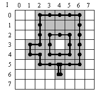
Contour Length differentiates between a 4-connected neighborhood and an 8-connected neighborhood. If the blob analysis operator is set to detect objects using a 4-connected neighborhood, the contour length is determined by scanning the edges of an object in orthogonal directions only. If the blob analysis operator is set to 8-connected neighborhood, the contour length also considers diagonally connected object edges. Thus, depending on the neighborhood setting of the operator, the feature provides two different results.
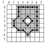
The two figures below illustrate the difference. Both figures show an image containing a single object.
In the upper figure, the object is detected using a 4-connected neighborhood. For this object, the contour length sums up all pixels located at object edges. Only horizontal and vertical pixel connections are considered. Therefore, the object results in a contour length of 30x orthogonal length.
In the lower figure, the blob analysis uses an 8-connected neighborhood. The contour length also considers diagonal edges. The object results in a contour length of 14x orthogonal length + 8x diagonal lengh.
The results differ in contour length.
The edge connecting two neighboring pixels diagonally has the contour length
 which represents the hypotenuse of an
isosceles triangle. This square root operation is not performed by the blob
analysis operators. Make sure it is performed afterwards in your design. The
total contour length can be obtained by
which represents the hypotenuse of an
isosceles triangle. This square root operation is not performed by the blob
analysis operators. Make sure it is performed afterwards in your design. The
total contour length can be obtained by
The diagonal component of the contour length is very important for objects with edges that run not in parallel to the image edges.
For example, a circle having a radius of 5.5 pixels will have a perimeter of
 . The figures
below show this circle. In the left-hand figure, the perimeter is calculated
using an 8-connected neighborhood. In the right-hand figure, the perimeter is
calculated using a 4-connected neighborhood. The example shows that the result
of the calculation using the 8-connected neighborhood (32.97) is close to the
theoretic result (34.56), The result of the calculation using the 4-connected
neighborhood (40) is rather poor - it is equal to the perimeter of a rectangle
having the same diameter.
. The figures
below show this circle. In the left-hand figure, the perimeter is calculated
using an 8-connected neighborhood. In the right-hand figure, the perimeter is
calculated using a 4-connected neighborhood. The example shows that the result
of the calculation using the 8-connected neighborhood (32.97) is close to the
theoretic result (34.56), The result of the calculation using the 4-connected
neighborhood (40) is rather poor - it is equal to the perimeter of a rectangle
having the same diameter.
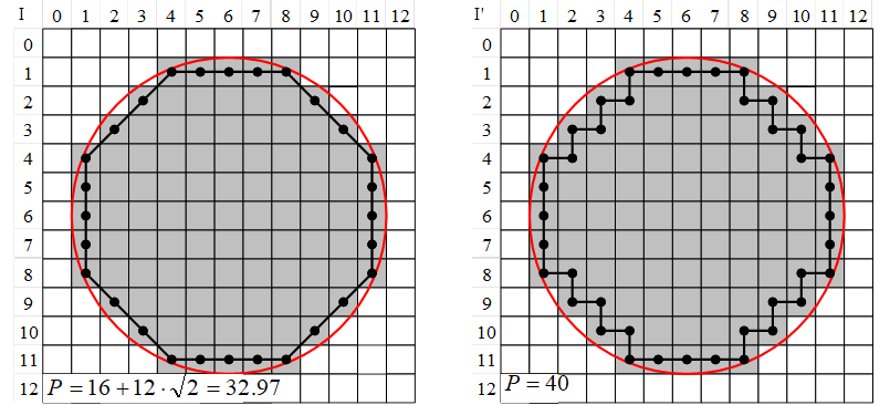
Figure 420. Calculation of the perimeter using an 8-connected neighborhood (left) and a 4-connected neighborhood (right)
